Note
Click here to download the full example code
Plot iterations of AMFClassifier
In this examples we illustrate the evolution of the decision function produced by
AMFClassifier along iterations (repeated calls to partial_fit).

Out:
Plotting iterations:   0%|          | 0/6 [00:00<?, ?it/s]
Plotting iterations:  17%|#6        | 1/6 [00:01<00:09,  1.83s/it]
Plotting iterations:  33%|###3      | 2/6 [00:03<00:07,  1.90s/it]
Plotting iterations:  50%|#####     | 3/6 [00:06<00:06,  2.02s/it]
Plotting iterations:  67%|######6   | 4/6 [00:08<00:04,  2.22s/it]
Plotting iterations:  83%|########3 | 5/6 [00:11<00:02,  2.46s/it]
Plotting iterations: 100%|##########| 6/6 [00:15<00:00,  2.72s/it]
Plotting iterations: 100%|##########| 6/6 [00:15<00:00,  2.54s/it]
import sys
import logging
import matplotlib.pyplot as plt
from tqdm import trange
from sklearn.datasets import make_moons
from sklearn.metrics import roc_auc_score
from sklearn.model_selection import train_test_split

sys.path.extend([".", ".."])
from onelearn import AMFClassifier
from experiments.plot import (
    get_mesh,
    plot_contour_binary_classif,
    plot_scatter_binary_classif,
)

logging.basicConfig(
    format="%(asctime)s %(message)s", datefmt="%Y/%m/%d %H:%M:%S", level=logging.INFO
)

norm = plt.Normalize(vmin=0.0, vmax=1.0)

n_samples = 400
n_features = 2
n_classes = 2
seed = 123
random_state = 42
levels = 30

save_iterations = [5, 10, 20, 50, 100, 200]
output_filename = "iterations.pdf"

logging.info("Simulation of the data")
X, y = make_moons(n_samples=n_samples, noise=0.2, random_state=random_state)

logging.info("Train/Test splitting")
X_train, X_test, y_train, y_test = train_test_split(
    X, y, test_size=0.5, random_state=random_state
)

logging.info("Computation of the meshgrid")
xx, yy, X_mesh = get_mesh(X)


clf = AMFClassifier(
    n_classes=n_classes,
    n_estimators=100,
    random_state=random_state,
    split_pure=True,
    use_aggregation=True,
)


n_plots = len(save_iterations)
n_fig = 0
save_iterations = [0, *save_iterations]

fig, axes = plt.subplots(nrows=2, ncols=n_plots, figsize=(3 * n_plots, 6))

logging.info("Launching iterations")
bar = trange(n_plots, desc="Plotting iterations", leave=True)


for start, end in zip(save_iterations[:-1], save_iterations[1:]):
    X_iter = X_train[start:end]
    y_iter = y_train[start:end]
    clf.partial_fit(X_iter, y_iter)

    ax = axes[0, n_fig]
    plot_scatter_binary_classif(
        ax,
        xx,
        yy,
        X_train[:end],
        y_train[:end],
        s=50,
        title="t = %d" % end,
        fontsize=20,
        noaxes=False,
    )

    Z = clf.predict_proba(X_mesh)[:, 1].reshape(xx.shape)
    score = roc_auc_score(y_test, clf.predict_proba(X_test)[:, 1])
    ax = axes[1, n_fig]
    plot_contour_binary_classif(ax, xx, yy, Z, score=score, levels=levels, norm=norm)
    n_fig += 1
    bar.update(1)

bar.close()

plt.tight_layout()
plt.savefig(output_filename)
logging.info("Saved result in file %s" % output_filename)
Total running time of the script: ( 0 minutes 16.269 seconds)

